Data Points
Collect acoustic measurements across time and frequency
Overview
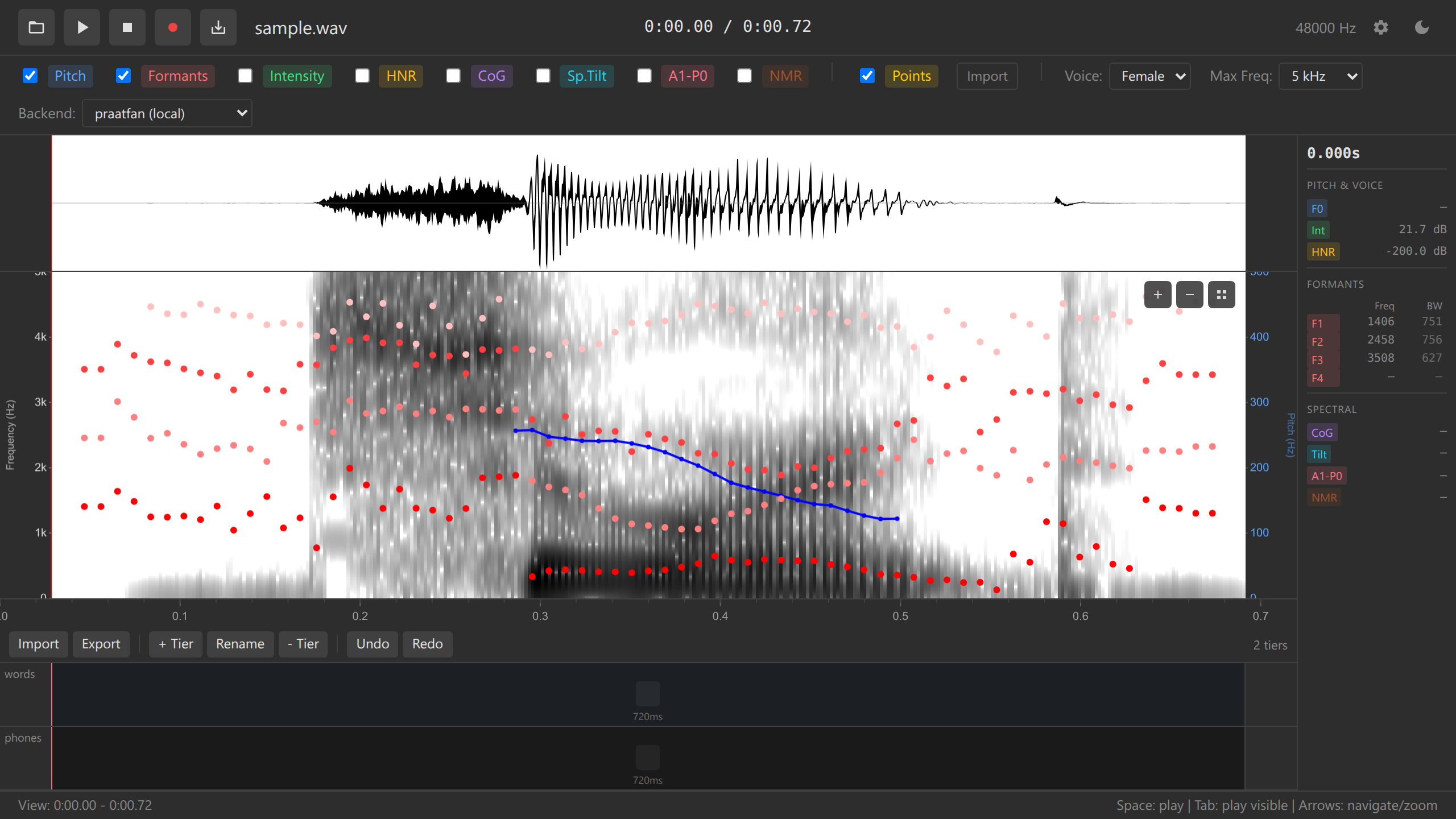
Data points enable systematic collection of acoustic measurements at specific time-frequency locations. Each point automatically captures all available acoustic values and annotation labels, making it ideal for vowel formant collection, prosody research, and quantitative phonetics.
Key Features
- Quick collection - Double-click to add measurement points
- Comprehensive measurements - Auto-captures all acoustic values
- Annotation integration - Includes labels from all annotation tiers
- Visual markers - Yellow dashed lines with position indicators
- Drag to move - Reposition points for precise measurement
- TSV export - Export to tab-separated values for analysis
- TSV import - Re-import previous measurements
- Undo support - Full undo/redo for add/move/remove operations
Adding Data Points
Via Double-Click
- Enable desired overlays (pitch, formants, etc.)
- Double-click on spectrogram at target location
- Yellow dashed line appears at that time
- Values panel shows measurements at that point
The vertical position of your double-click doesn’t affect measurements — it only sets the time position. All acoustic values (pitch, formants, intensity, etc.) are computed at that time point automatically.
Moving Data Points
Drag horizontally: 1. Click and hold data point marker (yellow line) 2. Drag left or right to new time position 3. Release to place 4. Measurements update automatically
Adding, moving, and removing data points are fully undoable with Ctrl+Z / Cmd+Z.
Removing Data Points
Right-click menu: 1. Right-click on data point marker 2. Select “Remove data point”
Collected Measurements
Each data point automatically captures:
Time-Frequency Position
- Time - Exact time position (seconds)
- Frequency - Cursor frequency at time of placement (Hz)
Acoustic Measurements
- Pitch (F0) - Fundamental frequency (Hz)
- Intensity - Sound pressure level (dB)
- Formants - F1, F2, F3, F4 (Hz)
- Bandwidths - B1, B2, B3, B4 (Hz)
- HNR - Harmonics-to-noise ratio (dB)
- CoG - Center of gravity (Hz)
- Spectral Tilt - Spectral slope
- A1-P0 - Nasal measure (dB)
Annotation Labels
- Automatic text from all annotation tiers at that time point
- Column per tier:
label_words,label_phones, etc.
Values Panel
Hover over any data point to see its measurements in the values panel:
📍 Data Point #1

Time: 1.234 s
Freq: 523 Hz

Pitch: 245 Hz
Intensity: 68 dB
F1:  720 Hz  B1:  80 Hz
F2: 1240 Hz  B2: 110 Hz
F3: 2650 Hz  B3: 150 Hz
F4: 3500 Hz  B4: 200 Hz
HNR: 15.3 dB
CoG: 5420 Hz

Annotations:
  words: "cat"
  phones: "æ"
TSV Export
Export all data points to tab-separated values format for statistical analysis.
Export Process
- Click “Export Data Points” button
- Choose save location
- File saves as
data-points.tsv
Quick copy to clipboard: - Press Ctrl+C (Windows/Linux) or Cmd+C (Mac) to copy all data points as TSV to clipboard - Paste directly into spreadsheet software or text editor - No file dialog needed
TSV Format
Header row:
time freq pitch intensity f1 f2 f3 f4 b1 b2 b3 b4 hnr cog spectral_tilt a1_p0 label_words label_phonesData rows:
1.234   720 245 68  720 1240    2650    3500    80  110 150 200 15.3    5420    -2.1    -5.4    "cat"   "æ"
1.567   850 250 70  850 1180    2580    3450    85  105 145 195 16.1    5380    -1.9    -4.8    "sat"   "æ"
Notes: - Tab-separated (TSV), not comma - Missing values: empty field - Text labels: quoted strings - Decimal separator: period (.)
Import into R
# Read TSV file
data <- read.table("data-points.tsv", header=TRUE, sep="\t", quote="\"")

# Plot F1 vs F2 vowel space
library(ggplot2)
ggplot(data, aes(x=f2, y=f1, label=label_phones)) +
  geom_text() +
  scale_x_reverse() +
  scale_y_reverse() +
  labs(title="Vowel Space", x="F2 (Hz)", y="F1 (Hz)")
Import into Python/Pandas
import pandas as pd
import matplotlib.pyplot as plt

# Read TSV file
df = pd.read_csv("data-points.tsv", sep='\t')

# Plot F1 vs F2
plt.scatter(df['f2'], df['f1'])
plt.gca().invert_xaxis()
plt.gca().invert_yaxis()
plt.xlabel('F2 (Hz)')
plt.ylabel('F1 (Hz)')
plt.title('Vowel Space')
plt.show()
Import into Praat
# Read table
table = Read Table from tab-separated file: "data-points.tsv"

# Extract columns
selectObject: table
f1 = Get column index: "f1"
f2 = Get column index: "f2"

# Plot
Scatter plot: "f2", 0, 3000, "f1", 0, 1000, "label_phones", 12, "yes", "+"
TSV Import
Re-import previously exported data points:
- Click “Load Data Points” button
- Select
.tsvfile - Data points appear on spectrogram
- File must have header row with column names
- Required columns:
time(other columns optional) - Audio must be loaded first
- Imported points overwrite existing points
Use Cases
Vowel Formant Collection
Goal: Measure F1/F2 for vowel categories
Workflow: 1. Load audio with vowels 2. Enable formants overlay 3. Add annotation tier for vowel labels 4. Double-click vowel midpoint for each token 5. Export TSV 6. Plot F1 vs F2 in R/Python
Result: Vowel space plot with formant ellipses per category
Pitch Contour Sampling
Goal: Sample pitch at specific phrase positions
Workflow: 1. Load audio with intonation of interest 2. Enable pitch overlay 3. Add annotation tier for prosodic events 4. Double-click at onset, peak, offset 5. Export TSV 6. Analyze pitch trajectory
Result: Quantitative intonation patterns
Fricative CoG Measurements
Goal: Measure spectral properties of fricatives
Workflow: 1. Load audio with /s/, /ʃ/ contrasts 2. Enable CoG overlay 3. Add phone-level annotations 4. Double-click fricative midpoints 5. Export TSV 6. Compare CoG distributions
Result: Acoustic distinction between sibilant categories
Voice Quality Time Series
Goal: Track HNR across utterance
Workflow: 1. Load audio 2. Enable HNR overlay 3. Add data points at regular intervals (every 50ms) 4. Export TSV 5. Plot HNR over time
Result: Voice quality trajectory showing modal/non-modal regions
Visual Appearance
Data points are displayed as:
- Vertical yellow dashed line - Extends full height of spectrogram
- Circle marker - At bottom of spectrogram
- Index number - Small label (1, 2, 3, …) for identification
Color customization:
# config.yaml
colors:
  dataPoint: "#FFFF00"  # Yellow (default)
Keyboard Workflow
Efficient keyboard-driven data collection:
| Key | Action |
|---|---|
| Double-click spectrogram | Add data point |
| Click data point | Select |
| Ctrl+Z / Cmd+Z | Undo add/move/remove |
| Ctrl+Y / Cmd+Shift+Z | Redo |
Rapid collection: 1. Play audio (Space) 2. Pause at target (Space) 3. Double-click spectrogram to add point 4. Repeat
Integration with Annotations
Data points automatically integrate with annotation tiers:
Example scenario:
Annotations:
  words:  | the   | cat       | sat       |
  phones: | ð | ə | k | æ | t | s | æ | t |

Data Points:
  Point 1 at 0.5s → captures "the", "ə"
  Point 2 at 1.2s → captures "cat", "æ"
  Point 3 at 1.8s → captures "sat", "æ"
TSV output:
time   f1   f2   label_words  label_phones
0.5    520  1720  "the"        "ə"
1.2    720  1240  "cat"        "æ"
1.8    850  1180  "sat"        "æ"
This enables within-category statistical analysis: “Compare F1 for all /æ/ tokens”
Performance
Data point operations enable rapid collection workflows.
Limitations
Current version: - All data points at time resolution (can’t select specific frequency for formant) - No visual connection between points (no trajectories) - TSV is the only export format (no CSV, JSON, XLSX)
Future enhancements: - Click-and-drag formant tracking - Visual trajectories connecting sequential points - Multiple export formats - Statistical summary export (means, SDs per category)
Troubleshooting
Data Point Not Appearing
Problem: Double-click doesn’t create point
Possible causes: - Not clicking on spectrogram (clicking annotation tier instead) - Spectrogram not loaded (for long files, zoom in first)
Solution: - Ensure spectrogram is visible - Double-click directly on spectrogram canvas - Zoom in if file is >60 seconds
Missing Values in Export
Problem: TSV has empty cells
Explanation: This is normal when: - Overlay not enabled (pitch values missing if pitch overlay off) - Unvoiced region (pitch undefined for /s/, /t/) - No annotation at that time (label columns empty)
Solution: - Enable all desired overlays before adding points - Accept missing values as linguistically meaningful - Filter during analysis (e.g., remove unvoiced tokens)
Can’t Move Data Point
Problem: Point won’t drag
Solution: - Click precisely on yellow line - Ensure not in text edit mode - Try zooming in for better precision
See Also
- Tutorial: Data Collection - Step-by-step guide
- Acoustic Overlays - Understanding measurements
- Annotations - Creating annotation labels
- Exporting - Export workflows